Mach 3 Wind Tunnel with a Forward-Facing Step: Wavelet-Adapted Mesh in OpenFOAM
Key result: with a mesh adapted by wavelet thresholding, rhoCentralFoam reproduces the Mach 3 forward-step flow of a uniform mesh four times finer to $0.031$ in density on average (against $0.160$ for the uniform base mesh), with $21\%$ of its cells in the plane. The wall-clock time, however, is $4.4$ times that of the fine uniform run: OpenFOAM's refinement splits the cells across the thickness of the 2D slab too, and changing the mesh every two time steps costs six times more per cell than the solver itself.
SUMMARY
The Mach 3 flow in a wind tunnel with a forward-facing step, the classical benchmark of Emery [ref. 3] and of Woodward and Colella [ref. 4], was computed with rhoCentralFoam, the density-based solver of the computational fluid dynamics (CFD) toolbox OpenFOAM [ref. 1], up to the time $t = 4$. The geometry and the base mesh, $4032$ square cells of size $h = 1/40$, were made with gmsh [ref. 8]. The mesh was then adapted during the computation: a function object computes, in every cell, the detail coefficients of an interpolating wavelet transform of the density and the pressure, and the cells whose coefficient exceeds $\varepsilon = 0.01$ (relative to the maximum of the field) are refined, twice, down to $h = 1/160$, while the others are coarsened. This is the principle of wavelet compression [refs. 5, 6, 7]: away from discontinuities the coefficients are small, and the solution there can be represented on coarse cells.
The adapted mesh follows the bow shock, the Mach stem, the reflected shocks and the slip line through the whole run, and its density field cannot be told apart from that of a uniform $1/160$ mesh ($64\,512$ cells). The mean density difference with this reference is $0.031$, five times smaller than for the uniform $1/40$ mesh ($0.160$); the bow shock is at the same place to within one fine cell. The adapted mesh holds $13\,735$ cells in the plane on average, $21.3\%$ of the reference. The gain in cells does not translate into a gain in time with the OpenFOAM implementation, for two reasons that are measured here. First, the refinement engine (hexRef8) splits each cell into eight, including across the slab thickness, so the adapted run carries $42\,633$ cells on average, $66\%$ of the reference, instead of $21\%$. Second, the mesh changes every two time steps, and each change costs more than a time step: the run costs $11.8$ core-microseconds per cell and step, against $2.0$ for the uniform mesh. The adapted run takes $3886\,\mathrm{s}$ on two cores, the fine uniform run $883\,\mathrm{s}$.
INTRODUCTION
In 1968 Emery compared several difference schemes on the supersonic flow in a wind tunnel partly blocked by a step [ref. 3]; Woodward and Colella made it a standard test for shock-capturing schemes in 1984 [ref. 4]. A uniform Mach 3 stream enters a tunnel and meets a step. A bow shock forms ahead of the step, reflects on the upper wall, then on the top of the step, and so on down the tunnel; a Mach stem grows at the upper wall, and a slip line (a contact discontinuity across which the velocity jumps) leaves its triple point. A centred expansion fan turns the flow around the corner of the step. The interest of the case is that it contains every kind of feature of a compressible flow, strong and weak shocks, contact discontinuity, expansion and a singular point, in a simple geometry.
Most of the domain, however, holds a smooth flow. A mesh fine enough for the shocks everywhere wastes most of its cells. Adaptive mesh refinement puts the fine cells where they are needed and moves them with the features. The difficulty is the criterion: where is the mesh "needed"? Wavelets give a systematic answer. The wavelet transform of a field separates it into a coarse approximation and detail coefficients at each scale; the detail coefficients are small where the field is smooth and large near discontinuities. Discarding the small ones (compression) leaves an approximation of known accuracy; refining the mesh only where the detail coefficients are significant is the corresponding adaptive method [refs. 5, 7].
The question of this study is how well such a wavelet-adapted mesh, built on OpenFOAM's standard adaptive refinement, reproduces the solution of a uniform fine mesh, and what it costs. Three runs are compared: the uniform base mesh ($h = 1/40$), the adapted mesh ($1/40$ to $1/160$) and the uniform fine mesh ($1/160$), which serves as the reference.
METHODOLOGY
The gas is inviscid and perfect, with $\gamma = 1.4$; the flow follows the Euler equations
$$ \begin{equation} \frac{\partial \rho}{\partial t} + \nabla \cdot (\rho \mathbf{u}) = 0, \qquad \frac{\partial \rho \mathbf{u}}{\partial t} + \nabla \cdot (\rho \mathbf{u} \otimes \mathbf{u}) + \nabla p = 0, \qquad \frac{\partial \rho E}{\partial t} + \nabla \cdot \left[ (\rho E + p) \mathbf{u} \right] = 0, \end{equation} $$
with $E = p / [(\gamma - 1) \rho] + |\mathbf{u}|^2 / 2$. The problem is dimensionless, in the units of Woodward and Colella: the gas constant is $R = 0.714$ and $c_p = 2.5$, so that the inflow state, $\rho = 1.4$, $p = 1$, $T = 1$, has a sound speed of $1$, and $u = 3$ is Mach 3.
Figure 1 represents the general setup of the problem. The tunnel is $3$ long and $1$ high; the step, $0.2$ high, starts at $x = 0.6$ and runs to the outlet. The inlet ($x = 0$) imposes the Mach 3 state. The outlet is supersonic: all quantities are extrapolated (zero gradient). The upper wall and the floor ahead of the step are symmetry planes, that is reflecting walls, and the step is a slip wall: the flow slides along the walls without friction. The initial state is the inflow state everywhere, as in ref. 4.
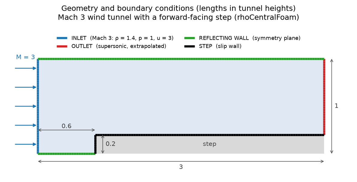
FIGURE 1. Geometry and boundary conditions (lengths in tunnel heights).
Mesh. The geometry is written in a gmsh script (step.geo) as three rectangles, meshed with structured quadrilaterals of side $h$ and extruded by one layer of thickness $h$, so that every cell is a cube. The base mesh, $h = 1/40$, has $4032$ cells (figure 2); the fine reference mesh, $h = 1/160$, is made by the same script and has $64\,512$ cells. The step corner falls on a grid line at every level, and every cell of a coarser or adapted mesh is exactly a union of cells of the fine mesh, so the runs are compared on the fine grid without any interpolation. The meshes are converted with gmshToFoam, and pass checkMesh with an aspect ratio of $1$ and no non-orthogonality.
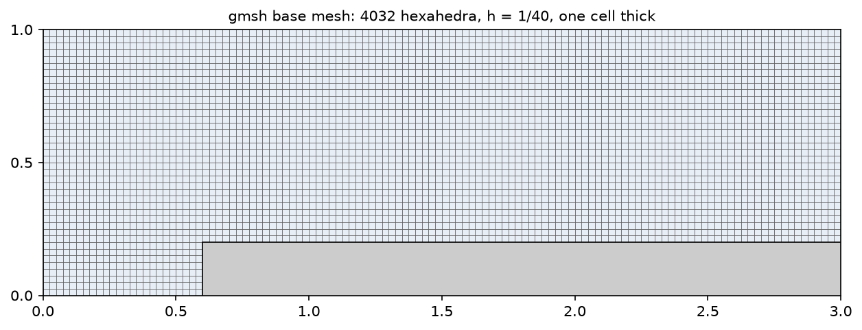
FIGURE 2. gmsh base mesh, $h = 1/40$, one cell thick.
Solver. rhoCentralFoam integrates equation $(1)$ with the central-upwind scheme of Kurganov and Tadmor [refs. 2, 9]: the fluxes are built from values reconstructed on both sides of each face with a van Leer limiter, weighted by the local wave speeds. The time step is set for a Courant number of $0.2$ (explicit Euler). The settings are those of the forwardStep tutorial of OpenFOAM. The runs use OpenFOAM v2506 in its official Docker image; the two fine runs use two MPI processes.
Wavelet detail coefficients
The adaptation is driven by a coded function object, waveletAMR, executed at every time step. In a lifting scheme [ref. 6], one level of a wavelet transform keeps every other sample as the coarse approximation, and replaces each remaining sample by its difference with a prediction from its coarse neighbours: this difference is the detail coefficient. With a linear prediction (the interpolating wavelet of order 2), and for a cell $P$ with neighbours $W$ and $E$ at distances $\Delta_W$ and $\Delta_E$ along $x$, the detail coefficient of a field $q$ is
$$ \begin{equation} d_x = q_P - \frac{\Delta_E \, q_W + \Delta_W \, q_E}{\Delta_W + \Delta_E}, \end{equation} $$
and likewise along $y$. The formula applies to irregular point sets, which is what an adapted mesh is: where a side has several smaller neighbours, their values and distances are averaged with the face areas as weights, and on a boundary the face value takes the place of the neighbour. Where $q$ is smooth, a Taylor expansion gives
$$ \begin{equation} d_x = -\tfrac{1}{2} \Delta_W \Delta_E \, \frac{\partial^2 q}{\partial x^2} + O(h^3), \end{equation} $$
so the coefficient falls by a factor of four each time the cell is halved; across a discontinuity of amplitude $[q]$, it stays of the order of $[q]/2$ however small the cells. Thresholding the coefficients therefore keeps the fine cells at the discontinuities and releases them elsewhere. The indicator of a cell is the largest of $|d_x|$ and $|d_y|$ for the density and for the pressure, each divided by the maximum of the field over the domain:
$$ \begin{equation} D_P = \max_{q \in \{\rho, p\}} \; \frac{\max(|d_x|, |d_y|)}{\max_\Omega |q|}. \end{equation} $$
A cell is significant when $D_P > \varepsilon$, with $\varepsilon = 0.01$ (system/waveletDict). As in Harten's multiresolution schemes [ref. 5], the significant set is extended by a safety zone, here two cells in every direction, so that a shock moving at most one cell between two adaptations stays in fine cells.
Adaptation. OpenFOAM's dynamicRefineFvMesh reads the dilated indicator every two time steps. It splits the significant cells (a cube into eight cubes, with hexRef8) up to two levels, $h = 1/160$, and merges back the groups of eight cells whose indicator has dropped below $\varepsilon / 2$ all around. The interval of two steps and the safety zone are consistent: at a Courant number of $0.2$, a shock moves at most $0.4$ cell in two steps. The refinement keeps a 2:1 ratio between neighbours. hexRef8 has no two-dimensional mode: it also splits the cells across the slab, so the adapted run uses symmetry planes instead of empty patches on the front and the back, and a cell of level 2 is a column of four cubes. The flow stays two-dimensional; the cost is counted below.
RESULTS
Figure 3 shows the density at $t = 4$ for the three meshes, with the 30 contour levels of Woodward and Colella. All three show the same structure. The bow shock stands at $x = 0.31$ on the floor; it is curved, and reaches the upper wall as a Mach stem, a nearly normal shock at $x \approx 0.6$, with a triple point at $y \approx 0.76$. From the triple point, the reflected shock runs down to the top of the step at $x \approx 1.32$, reflects back up, reaches the upper wall at $x \approx 2.42$, and reflects again. A slip line leaves the triple point and runs downstream near $y \approx 0.8$. The expansion fan centred on the corner of the step lowers the density to $0.02$ next to the corner.
On the uniform $1/40$ mesh, the shocks are spread over three to four cells, the slip line is smeared over a band $0.1$ wide, and the triple point is blunt. The adapted mesh and the fine uniform mesh give sharp shocks and the same contours; the only visible differences are the fine wiggles of the contours downstream, where the density is nearly uniform.
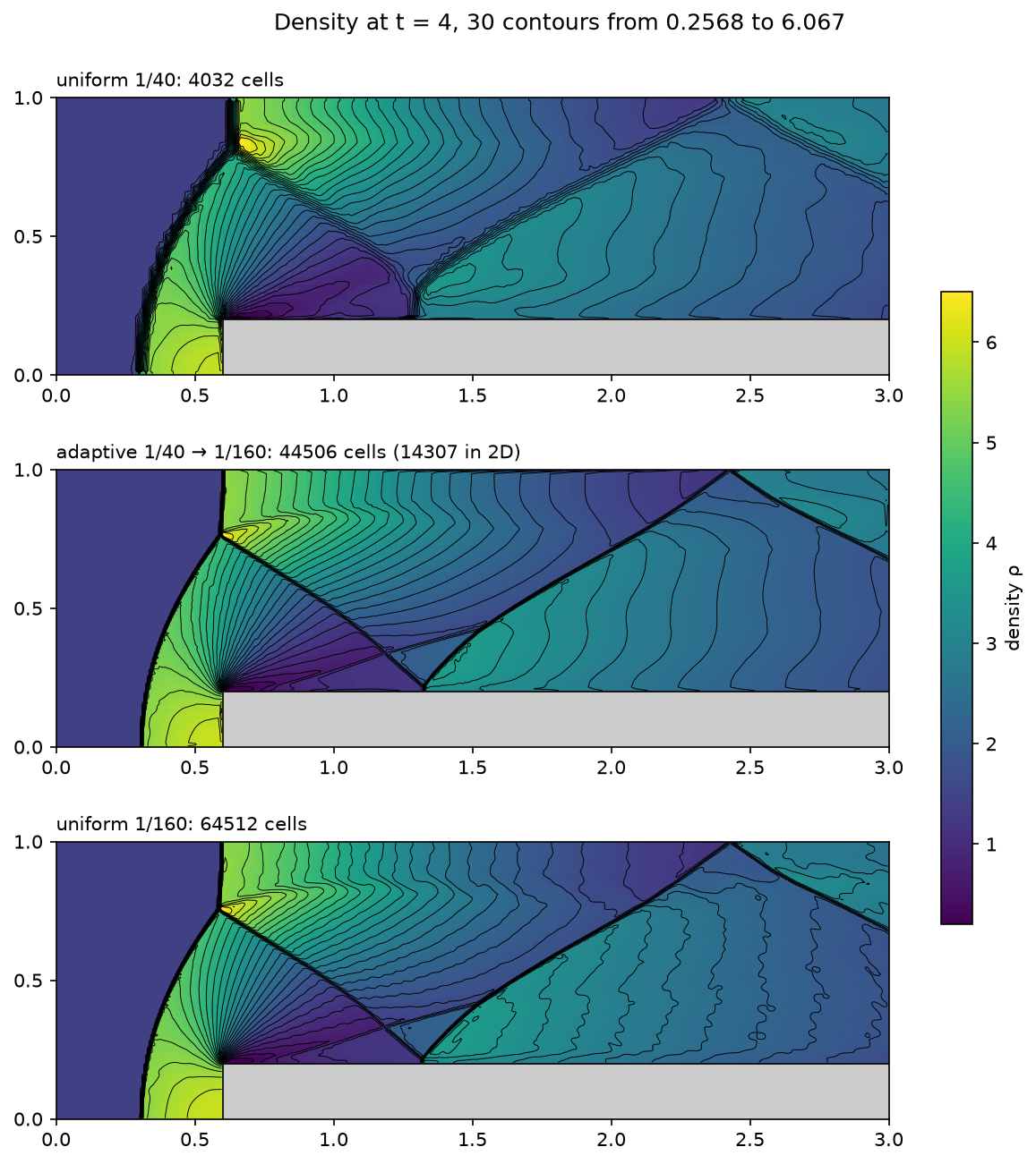
FIGURE 3. Density at $t = 4$ with 30 contours from $0.2568$ to $6.067$. Top: uniform $1/40$. Middle: adapted. Bottom: uniform $1/160$.
Figures 4 to 6 show the other fields of the adapted solution at $t = 4$. The pressure (figure 4) jumps across the bow shock from $1$ to about $10$, the value of a normal shock at Mach 3 ($p_2 / p_1 = 10.33$), and rises further to $12.2$ in front of the step, where the flow stops: the pitot pressure behind a normal shock at Mach 3 is $12.06$. The expansion around the corner drops it to $0.013$. The pressure is continuous across the slip line, which is therefore invisible in figure 4, unlike in the density.
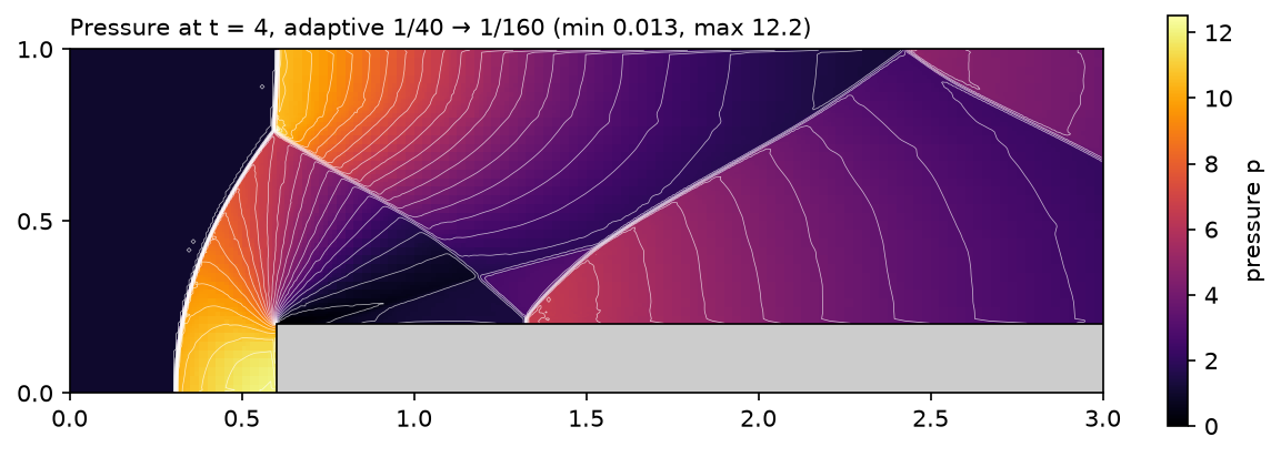
FIGURE 4. Pressure at $t = 4$, adapted mesh.
The temperature (figure 5) reaches $2.81$ in front of the step, the stagnation temperature of the inflow, $T_0 = 1 + \tfrac{\gamma - 1}{2} M^2 = 2.8$: the gas brought to rest there has converted all its kinetic energy into heat. Unlike the pressure, the temperature jumps across the slip line, which appears as the boundary between the warmer gas that went through the Mach stem and the cooler gas that went through the curved bow shock and the reflected shock. The lowest temperature, $0.34$, is in the corner expansion; the fine uniform mesh gives $0.50$ there. The corner is a singular point of the flow, where neither mesh gives a converged value.
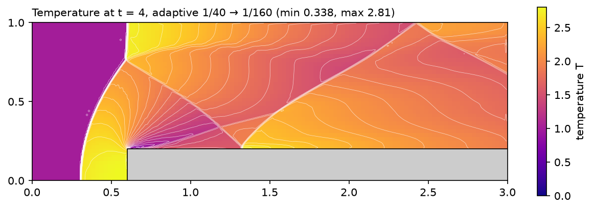
FIGURE 5. Temperature at $t = 4$, adapted mesh.
Figure 6 shows the speed and the streamlines. Behind the bow shock, the flow slows down to subsonic speeds and turns upwards to pass the step; in front of the step face it is nearly at rest. It accelerates again around the corner, up to $3.27$, faster than the inflow, then is turned back parallel to the walls by each shock it crosses.
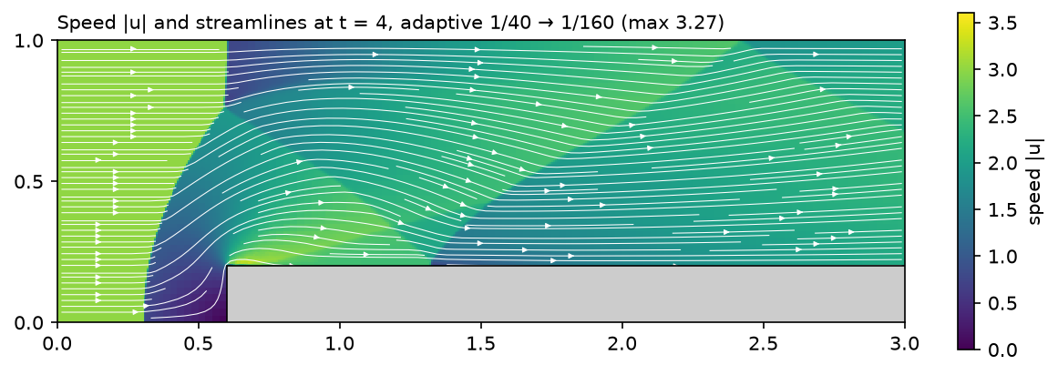
FIGURE 6. Speed $|\mathbf{u}|$ and streamlines at $t = 4$, adapted mesh.
These fields match the fine uniform solution as closely as the density. The mean difference with it is $0.047$ in pressure, $0.016$ in temperature and $0.019$ in speed for the adapted mesh, against $0.264$, $0.066$ and $0.083$ for the uniform $1/40$ mesh: about $1\%$ of the mean value for the adapted mesh, four to six times less than for the coarse one.
Figure 7 shows the adapted mesh at $t = 4$. The fine cells form bands of about eight cells around the bow shock, the Mach stem, the reflected shocks and the slip line; the rest of the domain, upstream of the bow shock and in the smooth flow between the shocks, is at the base size. Inside the expansion fan, patches of intermediate cells come and go: the density gradient is steep there, and the coefficient of equation $(3)$ hovers around the threshold. Figure 8 shows the cells in two close-ups: around the bow shock and the step corner, and around the triple point.
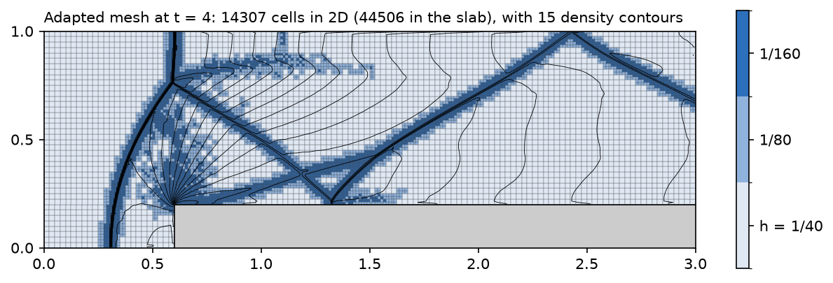
FIGURE 7. Adapted mesh at $t = 4$, coloured by level, with 15 density contours: $14\,307$ cells in the plane ($44\,506$ in the slab).
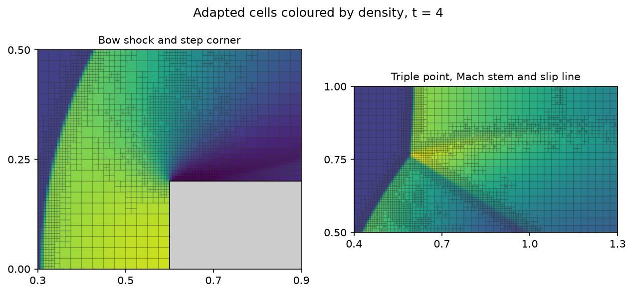
FIGURE 8. Close-ups of the adapted cells, coloured by density, at $t = 4$.
Figure 9 follows the mesh in time. At $t = 0.5$ the bow shock has not yet reached the upper wall; at $t = 1$ it reflects on it regularly; by $t = 2$ the reflection has become a Mach reflection with a stem and a slip line, and the reflected shock hits the step. At each time, the fine cells are where the shocks are, and nowhere else: the coarsening releases the cells behind a moving shock, so the mesh does not keep a trace of the past positions of the shocks.
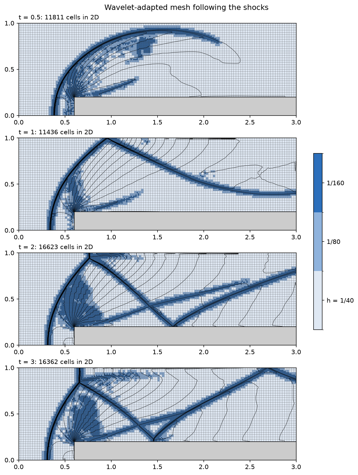
FIGURE 9. Adapted mesh at $t = 0.5$, $1$, $2$ and $3$.
The video shows the whole run, from $t = 0$ to $4$, one frame every $0.02$: the density above and the adapted mesh below. The bands of fine cells travel with the shocks, appear where a new reflection forms, and dissolve behind the shocks as the flow becomes smooth again.
VIDEO 1. Density (top) and wavelet-adapted mesh (bottom) from $t = 0$ to $4$.
Figure 10 gives the number of cells. In the plane, the adapted mesh rises to about $12\,000$ cells as the bow shock forms, then to $16\,000$ when the reflections fill the tunnel; it averages $13\,735$ cells over the run, $21.3\%$ of the uniform $1/160$ mesh, with a maximum of $18\,164$ ($28\%$). The count oscillates by about $\pm 1000$ cells from one adaptation to the next: cells in the expansion fan are refined and coarsened in turn. In the slab, because hexRef8 also splits in $z$, the adapted run carries $42\,633$ cells on average and $60\,984$ at most, close to the $64\,512$ of the uniform fine mesh.
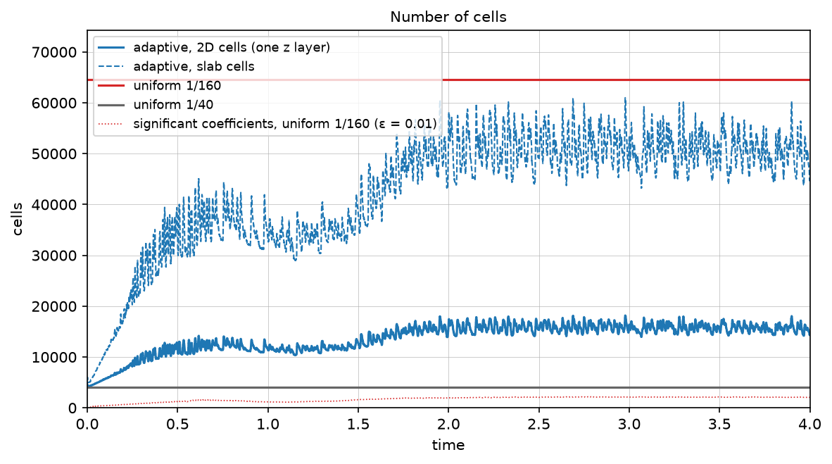
FIGURE 10. Number of cells against time. Solid blue: adapted, in the plane. Dashed blue: adapted, in the slab. Red: uniform $1/160$. Grey: uniform $1/40$. Dotted red: cells of the uniform $1/160$ run whose detail coefficient is above $\varepsilon$.
How far could the compression go? Figure 11 shows the detail coefficients of the fine uniform solution at $t = 4$. They span six orders of magnitude: above $0.1$ on the shocks, around $10^{-2}$ on the slip line and in the expansion fan, and $10^{-3}$ to $10^{-5}$ in the smooth regions. Only $3.2\%$ of them exceed $\varepsilon = 0.01$. The adapted mesh uses $21\%$ of the cells: the rest is the price of the safety zone, of the 2:1 grading, and of refining whole groups of cells around each significant one. The compression curve also shows how $\varepsilon$ controls the trade-off: the fraction of significant coefficients falls by about a factor of five per decade of $\varepsilon$, from $15.6\%$ at $10^{-3}$ to $3.2\%$ at $10^{-2}$ and $0.5\%$ at $10^{-1}$.
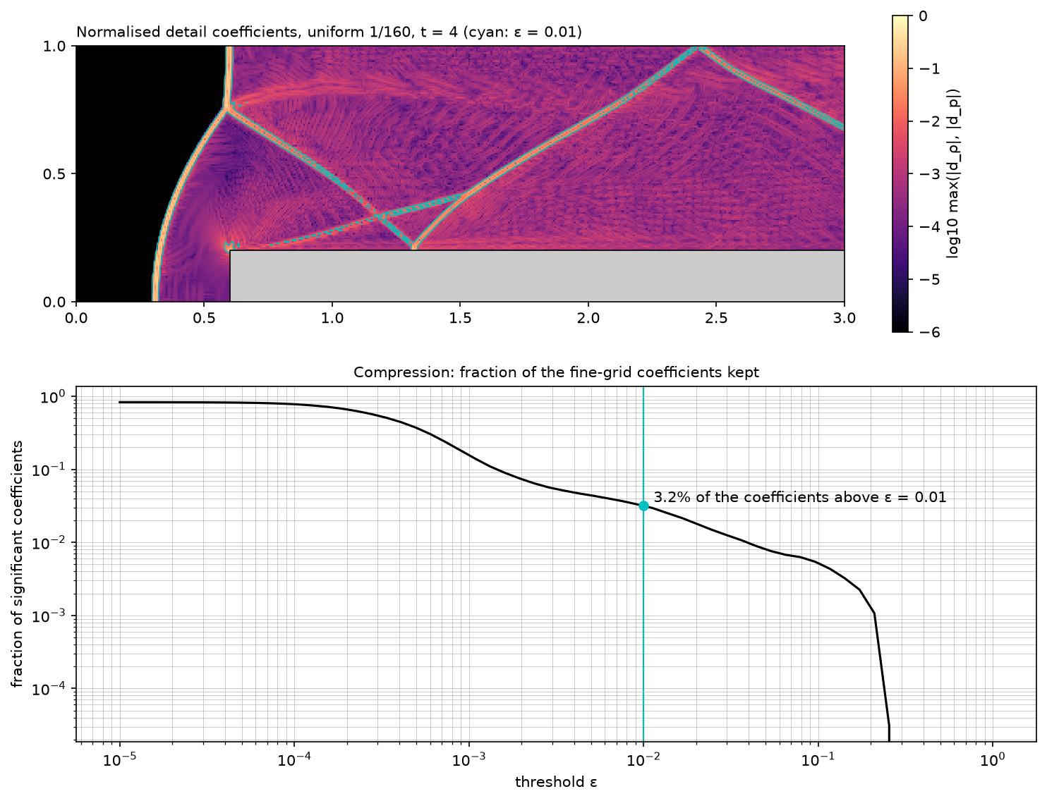
FIGURE 11. Top: normalised detail coefficients $D_P$ of the uniform $1/160$ solution at $t = 4$ (logarithmic scale; cyan: $D_P = \varepsilon$). Bottom: fraction of the coefficients above a threshold.
Figure 12 maps the density difference with the fine uniform solution. For the uniform $1/40$ mesh it is $0.160$ on average; it exceeds $1$ along the shocks, which are thicker and slightly displaced, and $0.2$ to $0.4$ in wide bands along the slip line and near the top of the step. For the adapted mesh it is $0.031$ on average, and remains only as thin lines along the shocks, where a difference of a fraction of a cell in position gives a large difference in density, and along the slip line. $95\%$ of the domain is within $0.091$ of the reference, against $0.717$ for the uniform $1/40$ mesh; the difference exceeds $0.5$ in $0.31\%$ of the domain, against $6.1\%$.
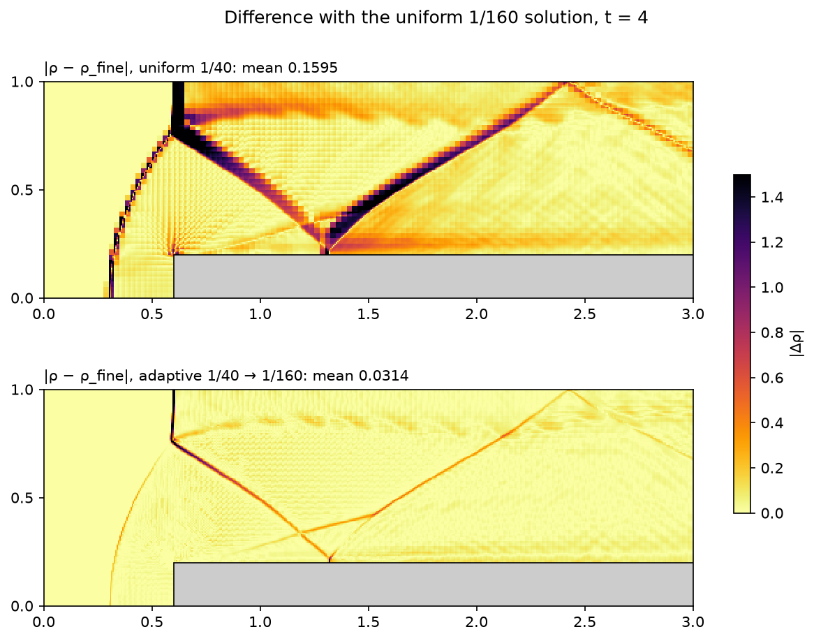
FIGURE 12. Density difference with the uniform $1/160$ solution at $t = 4$. Top: uniform $1/40$. Bottom: adapted.
Figure 13 compares density profiles. Along $y = 0.5$ the adapted and fine solutions coincide through the bow shock ($x = 0.43$), the reflected shock ($x = 0.99$) and the shock reflected from the step ($x = 1.64$); the uniform $1/40$ mesh spreads the last two over $0.05$ to $0.1$ and displaces them, by up to $0.1$ for the shock reflected from the step. Along $x = 2.4$, the slip line ($y \approx 0.83$) and the reflected shock near the wall show the same picture. The positions of the bow shock, taken where the density first exceeds $2.5$, agree to within one fine cell between the adapted and fine meshes ($0.353$ and $0.347$ at $y = 0.3$; $0.597$ and $0.591$ at $y = 0.8$), while the uniform $1/40$ mesh places it at $0.628$ at $y = 0.8$, $0.037$ downstream.
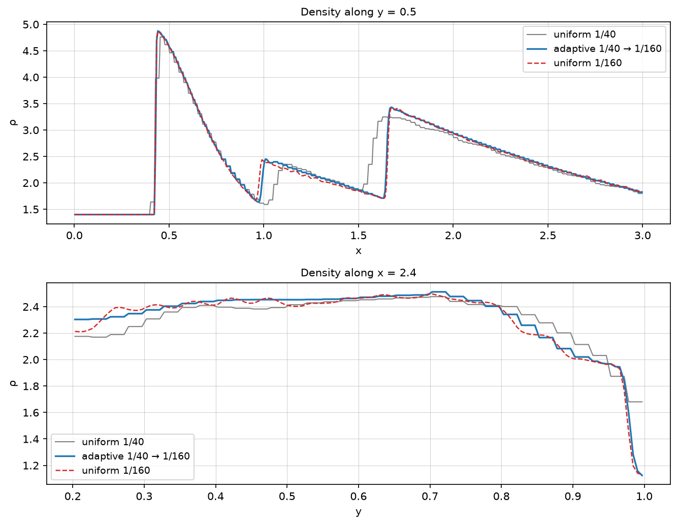
FIGURE 13. Density along $y = 0.5$ (top) and along $x = 2.4$ (bottom).
Cost. The table gathers the figures of the three runs.
| Uniform $1/40$ | Adapted $1/40 \to 1/160$ | Uniform $1/160$ | |
|---|---|---|---|
| Cells in the plane, end (mean) | $4032$ | $14\,307$ ($13\,735$) | $64\,512$ |
| Cells in the slab, end (mean) | $4032$ | $44\,506$ ($42\,633$) | $64\,512$ |
| Time steps | $3124$ | $15\,486$ | $13\,692$ |
| Mesh changes | $7568$ refinements, $7577$ coarsenings | ||
| Solver time | $32\,\mathrm{s}$, 1 core | $3886\,\mathrm{s}$, 2 cores | $883\,\mathrm{s}$, 2 cores |
| Cost per cell and step | $2.5\,\mu\mathrm{s}$ | $11.8\,\mu\mathrm{s}$ | $2.0\,\mu\mathrm{s}$ |
| Mean $|\rho - \rho_\mathrm{fine}|$ | $0.160$ | $0.031$ | |
| 95th percentile of $|\rho - \rho_\mathrm{fine}|$ | $0.717$ | $0.091$ | |
| Bow shock $x$ at $y = 0.8$ | $0.628$ | $0.597$ | $0.591$ |
The adapted run takes $4.4$ times longer than the fine uniform run, for three reasons. First, the cells across the slab: $42\,633$ cells on average instead of $13\,735$, a factor of $3.1$. Second, the time step: it is set by the smallest cells, which are the same as in the fine run; the adapted run even takes $13\%$ more steps, because a step that follows a refinement starts with a Courant number up to twice the target. Third, the mesh changes: every two steps hexRef8 rebuilds the mesh addressing and maps every field onto the new cells, which brings the cost to $11.8$ core-microseconds per cell and step against $2.0$ for a static mesh. This figure also includes the indicator (two loops over the faces per step) and the imbalance between the two processes: the domain is split once at the start, and dynamicRefineFvMesh does not redistribute the cells as the refinement moves. The runs do not separate these three contributions.
CONCLUSION
The Mach 3 forward-facing step was computed with rhoCentralFoam on gmsh meshes, with the goal of testing a mesh adapted by wavelet thresholding against uniform meshes. The detail coefficients of a linear interpolating wavelet, computed from each cell and its face neighbours, behave as the theory says: they fall as $h^2$ in the smooth flow and stay of the order of the jump at the shocks. Thresholded at $1\%$ of the field maximum, with a safety zone of two cells, they keep the fine cells on the bow shock, the Mach stem, the reflected shocks and the slip line throughout the run, and release them behind the moving shocks. The adapted solution matches the uniform $1/160$ solution to $0.031$ in density on average, five times better than the uniform $1/40$ mesh, with $21\%$ of the cells in the plane.
The accuracy is that of the fine mesh; the speed-up is not there, and the reason is the implementation, not the wavelet criterion. OpenFOAM's refinement is three-dimensional: in a 2D case it multiplies the adapted cells by up to four across the slab, which brings the average count to $66\%$ of the fine mesh. And changing the mesh every two steps, on a domain decomposition that is never rebalanced, multiplies the cost per cell and step by six. Three changes would recover the expected gain. A refinement restricted to the plane (as in the 2D refinement extensions of OpenFOAM, or in a cell-based adaptive code) would remove the factor of three. Adapting every five to ten steps, with a safety zone widened in proportion, would divide the overhead accordingly. And a local time step per refinement level would let the coarse cells, which are $80\%$ of the domain, take steps four times larger. In three dimensions, where hexRef8 is designed to work and a uniform fine mesh costs the cube of the refinement ratio, the same criterion would pay off directly. The threshold sets the trade-off: on this flow, $3\%$ of the coefficients of the fine solution exceed $\varepsilon = 0.01$, and each decade of $\varepsilon$ changes that fraction by about a factor of five.
REFERENCES
- OpenFOAM, version v2506, solver rhoCentralFoam and dynamicRefineFvMesh.
- C. J. Greenshields, H. G. Weller, L. Gasparini and J. M. Reese, "Implementation of semi-discrete, non-staggered central schemes in a colocated, polyhedral, finite volume framework, for high-speed viscous flows", International Journal for Numerical Methods in Fluids, 63, 2010, pp. 1-21.
- A. F. Emery, "An evaluation of several differencing methods for inviscid fluid flow problems", Journal of Computational Physics, 2, 1968, pp. 306-331.
- P. Woodward and P. Colella, "The numerical simulation of two-dimensional fluid flow with strong shocks", Journal of Computational Physics, 54, 1984, pp. 115-173.
- A. Harten, "Multiresolution algorithms for the numerical solution of hyperbolic conservation laws", Communications on Pure and Applied Mathematics, 48, 1995, pp. 1305-1342.
- W. Sweldens, "The lifting scheme: a construction of second generation wavelets", SIAM Journal on Mathematical Analysis, 29, 1998, pp. 511-546.
- O. V. Vasilyev and C. Bowman, "Second-generation wavelet collocation method for the solution of partial differential equations", Journal of Computational Physics, 165, 2000, pp. 660-693.
- C. Geuzaine and J.-F. Remacle, "Gmsh: a 3-D finite element mesh generator with built-in pre- and post-processing facilities", International Journal for Numerical Methods in Engineering, 79, 2009, pp. 1309-1331.
- A. Kurganov and E. Tadmor, "New high-resolution central schemes for nonlinear conservation laws and convection-diffusion equations", Journal of Computational Physics, 160, 2000, pp. 241-282.